Ask the Doctors: Analysis of Dynamic Range Control (DRC) Devices
Dr. Dave Berners

For the second month in a row, we will use this column to give a tutorial, rather than to focus on a particular question. This month's topic is analysis of dynamic range control (DRC) devices. We will take a look at what we need to know about a limiter/compressor in order to accurately characterize its behavior.

Automatic Gain Control
The behavior of dynamic range control devices is typically characterized with the following three pieces of information:

• attack time,
• release time, and
• static compression curve, or "compression knee."

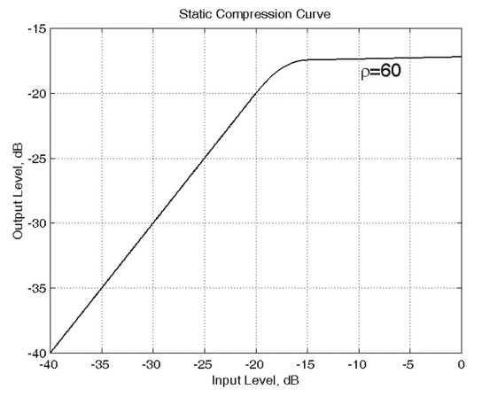
Attack- and release-time settings determine how quickly a device reacts to changes in input signal level. The static compression curve relates input levels to output levels for the device for steady-state signals (usually sine waves). Fig. 1 shows a typical static compression curve for a compressor with a ratio of 60:1 and a soft knee.

It is relatively well known that, for compressors/limiters with program dependence, the attack and release times are not constant; rather, they depend upon the statistics of the input signal. Usually, release times decrease for signals with a high peak-to-RMS ratio, to prevent dropouts following transients. For signals with higher RMS levels, release times increase, to prevent distortion caused by excessive gain modulation. Thus, a description that includes only the three pieces of information listed above is not complete for DRC devices with program dependence-and it is less well known that, even for DRC devices without program dependence, functional descriptions cannot be obtained solely from these three pieces of information. In other words, attack time, release time, and compression curves are not sufficient to characterize a DRC device properly, even if the device does not have program dependence.

“Attack time, release time, and compression curves are not sufficient to characterize a DRC device properly, even if the device does not have program dependence.”

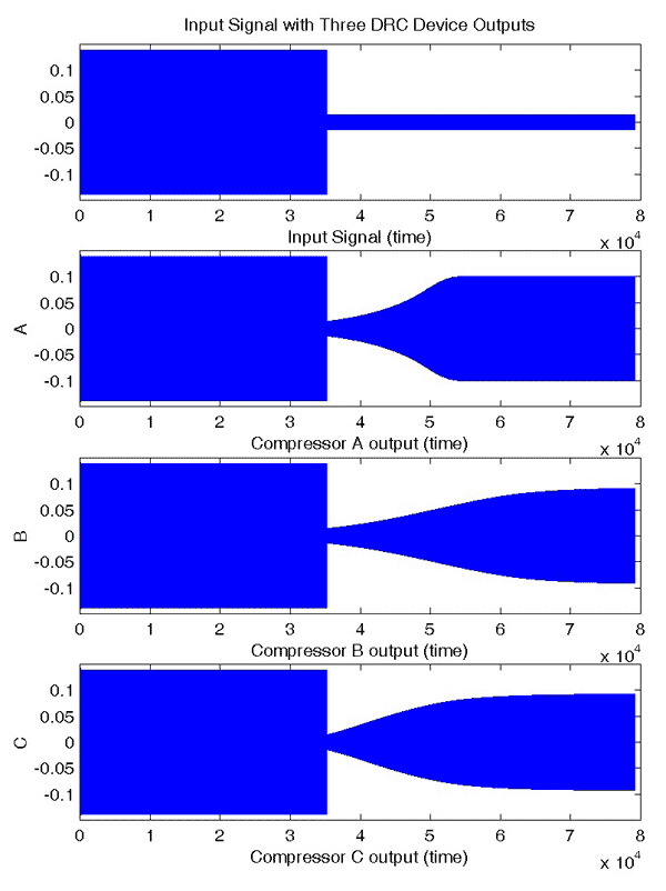
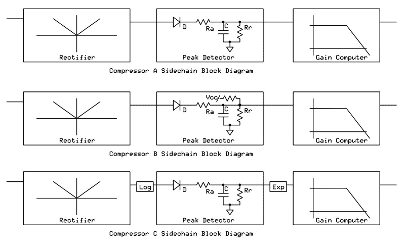
Fig. 2 shows the response of three different compressors to the same input signal. None of the compressors have program dependence, and all three of the compressors have the static compression curve shown in Fig. 1. As you can see, each of the release curves is different, even though all three compressors have the same release time. Fig. 3 shows block diagrams for the three compressors. All three use a peak detector consisting of a full-wave rectifier followed by an envelope follower. Compressors A and B differ only in the biasing of the envelope detector, with the quiescent estimate in B being biased at the threshold of compression. Compressor C has a similar envelope follower, but works in the log domain. All three compressors are feedforward and have the same gain computer, producing the static compression curve of Fig. 1.

It is easy to see that we could produce an infinite number of different compressors, each with different behavior, by changing the specifics of the level detection. Use of feedback topologies, RMS or other types of signal detection, and higher-order (program-dependent) detection can further increase the possible range of behavior exhibited by a DRC device. For this reason, it is very helpful to have an understanding of the internal structure of a device when trying to model its behavior.

When making measurements on a hardware DRC device, it is critical to know how the behavior at the output of the signal detector relates to the gain of the device. Many times, the attack and release circuitry contains linear components for the filtering. By measuring the output of the detector as related to the overall gain, nonlinearities on either side of the detector can be measured separately. Since nonlinearities cannot be commuted across the filter, the pre- and post-filtering nonlinearities must be kept segregated when implementing a model. Modeling the pre-detector and post-detector nonlinearities separately allows for distinctions such as those between compressors A, B and C of Fig. 2. To get the data to create such a model, measurements must be taken at the output of the detector, as well as at the output of the DRC device.

Audio Path Nonlinearities
Apart from nonlinearities in the sidechain, which are necessary to provide automatic gain control, there are often nonlinearities in the audio path of a DRC device. These nonlinearities can add audible harmonic distortion to the audio signal. In many cases, the amount and type of distortion is correlated with the amount of gain reduction being applied. However, this distortion is not considered an artifact of DRC if it exists even when the amount of gain reduction is held constant. The most obvious way to measure and characterize this distortion is to disconnect the sidechain of the device from the audio path and drive it with a constant signal so that you can control the amount of gain reduction independently. Then the amount and type of distortion can be measured as a function of gain reduction. It is critical to hold the amount of gain reduction constant so that distortion caused by audio path nonlinearities can be separated from modulation distortion caused by time-varying gain. Usually, even if the source of audio-path distortion is memoryless, it will not appear that way at the output, due to the fact that the audio channel is band limited. Some filtering almost always occurs both before and after the nonlinearities. This filtering must be modeled and inverted before the nonlinearities can be recovered. Alternatively, if the nonlinearities are memoryless and confined to one area of the circuit, the system can be modeled as a certain type of Volterra system. However, this method of analysis requires more data collection and has lower accuracy than modeling the linear and nonlinear portions of the circuit separately.

There are guidelines in the RCA Radiotron Designer's Handbook (which is very big to be called a handbook) and other sources that give the levels at which distortion becomes perceptible. An often-quoted figure for music is 0.7% of total harmonic distortion, assuming a balance of distortion components similar to what is produced by a pentode in Class A. For perceptibility, harmonic distortion should be weighted by the harmonic number; for example, fourth-harmonic distortion would be perceptible 6 dB below second-harmonic distortion. Note that when for sine tones, the levels for perceptibility are significantly lower; we are more sensitive to distortion when listening to sine waves than when listening to music.

Another factor that influences perceptibility is time span. We are not as sensitive to nonlinearities localized in time to a period shorter than 5 ms. So a DRC device may distort during transients, but if the attack time is less than 5 ms and the distortion does not continue after the attack is completed, we may not be overly sensitive to the distortion. An exception is the case when the distortion changes the amount of energy in the signal. When the amount of energy in a signal is changed by some form of distortion, the distortion is readily apparent to the listener, even if the distortion continues for only a short time.

Once audio path nonlinearities in a DRC device are recorded as a function of the amount of gain reduction, they can be added into the audio path. If the system is being modeled digitally, inclusion of distortion will require oversampling to avoid aliasing. A rule of thumb is that, if the nonlinearity can be modeled with an Nth-order power series, the oversampling factor must exceed N/2+1. Oversampling may have to be used to prevent aliasing from modulation distortion as well. For modulation distortion, if the device is feedforward, the gain signal and audio input may be upsampled by a factor of two separately before being multiplied.

In general, even heavily nonlinear systems can be modeled accurately with moderate DSP expense, provided those systems can be broken into memoryless nonlinearities and linear filters. If, however, systems are modeled as black boxes containing interspersed linear filters and memoryless nonlinearities in an unknown configuration, modeling becomes extremely difficult. The task of characterizing such a system based on static input-output level relationships and response times becomes effectively hopeless.