Volume 4, Number 3, April 2006
[UA Universe] [Ask the Doctors] [Artist Interview] [Analog Obsession]
[Support Report] [The Channel] [Plug-In Power] [Playback] [Featured Promotion]
[Graphic-Rich WebZine]
[Back Issues] [UA Home]
By Dr. Jonathan Abel
| Spring reverbs do have a sound all their own, and the question of what makes them sound "springy" came up as the UA engineers were modeling the spring in the Roland RE-201. The short answer has to do with how certain vibrations propagate along a spring: The low frequencies outrun the high frequencies. In this month's column, I'll talk about the details of this dispersive propagation and how it leads to the unique sound of a spring reverb. I'll also touch on some of the signal processing we did to emulate the spring in the RE-201 Space Echo.
“The problem of delaying different frequency bands different amounts is not so easily solved” Waves can propagate on springs in a number of ways; a few examples are shown in Figure 1. If you stretch a spring along its length, a restoring force develops to pull the spring back to its original shape. In this process, longitudinal waves propagate along the spring. If a spring is displaced away from its axis, a restoring force toward the axis develops, resulting in a transverse wave, much like what happens on a stretched string. If you twist a spring around its axis, the twisted coils will wind (or unwind, depending on the direction of the twist), causing adjacent coils to wind, and sending a torsional wave down the length of the spring. |
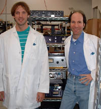 Dr. David Berners (left) is the Universal Audio Director of Algorithm Development; Dr. Jonathan Abel is the co-founder and CTO Dr. David Berners (left) is the Universal Audio Director of Algorithm Development; Dr. Jonathan Abel is the co-founder and CTO |
 |
|
Figure 1. Longitudinal (a), transverse (b), and torsional (c) propagation modes.
|
These different propagation modes have different propagation speeds, and by driving one end of the spring, the driving signal will appear delayed at the other end of the spring. As early as the 1920s, springs were used to delay audio signals for telephone applications such as echo cancellation.
In the late 1930s, Hammond - yes, that Hammond! - configured springs so that propagating waves would be reflected back and forth, creating a series of echoes reminiscent of reverberation. This idea is illustrated in Figure 2, a drawing from Hammond's 1941 patent. Modern day spring reverbs (such as the Accutronics springs found in many guitar amps) take a very similar approach, often using two or three springs at different tensions in parallel to increase echo density.
 |
|
Figure 2. Drawing from Hammond's 1941 spring reverb patent.
|
Now, consider the spring shown in Figure 3. It is stretched between two supports and has a magnetic bead attached to each end. The bead at the "driver" end is rotated according to a driving signal, and the resulting torsional wave propagates along the length of the spring. When the wave reaches the "pick-up" end of the spring, it will twist against the support and eventually be reflected back along the spring toward the driver. A pick-up detecting the rotation of the pick-up bead will therefore see a series of echoes in response to driver signals.
 |
|
Figure 3. Single spring with a driver and pick-up.
|
If we use T to denote the time it takes a signal to travel from the driver to the pick-up, we expect to see arrivals at T, 3T, 5T, and so on. In other words, the first arrival should be at T, and each successive arrival, 2T later. Successive echoes are expected to be quieter, as some signal energy is lost to damping with each end reflection, and some energy is lost to heat as the coils wind and unwind with the passing wave.
So what do we get if we measure the impulse response of a spring? Well, it's not just a tidy series of decaying echoes. As you can see in the example of Figures 4 and 5a, there is a bit more going on. The echoes are very smeared out in time, so much so that they overlap with adjacent echoes. Note that during each echo, low frequencies arrive first and high frequencies appear later. This is more clearly seen in the spectrogram of Figure 5b, which shows arrival energy as a function of time and frequency. Low-frequency signals appear to propagate much faster than high-frequency signals, making each arrival a sort of chirp. It is as if the spring were longer for higher frequencies. For instance, look at the arriving energy at 1 kHz. It is a series of echoes every 55 ms. At 2 kHz, the echoes arrive every 60 ms or so, and at 3 kHz, they appear about every 80 ms.
 |
|
Figure 4. Single spring impulse response.
|
 |
|
Figure 5. Single spring impulse response onset and spectrogram.
|
Looking at the spectrogram in Figure 5b, one other thing seems important, and perhaps not expected: The measured impulse response has very little energy above about 4 kHz. The transition is abrupt, and you can think of the impulse response equalization as including a high-cut filter.
To get an idea of what the 4 kHz is all about, consider the wavelength of signals traveling on the spring. A sine wave propagating trosionally on the spring would consist of bands of wound and unwound coils, as shown in Figure 1c. If the sine wave has a low frequency, the bands would encompass a large number of coils, each rotated a small amount relative to its neighbor. Above a sufficiently high frequency, however, the wave would span just a single coil, and would require adjacent coils to take on very different shapes. Under these circumstances, the nature of wave propagation is changed, and from the spectrogram of Figure 5b, it seems that torsional waves slow as frequency increases, and don't propagate above a cutoff frequency.
As an aside, dispersive propagation is common on strings. On piano strings, for instance, the high frequencies slightly outrun the low frequencies, making the higher harmonics a little sharp. This effect is more pronounced in the lower octaves, where the strings are thicker. Because propagation speed increases with frequency, transverse waves on piano strings don't have a cutoff frequency like torsional waves on springs do: If waves propagate slower and slower with increasing frequency, eventually the propagation speed goes to zero.
Now, take a listen to spring.wav; it contains the impulse response of a single idealized spring. You might be able to hear the impulse response as a series of chirps. The file chirp.wav is the same impulse response with the echoes composing it separated in time. As the impulse travels back and forth on the spring, it spreads out, and each successive echo lasts a little longer than the previous one.
You would probably hear a similar series of chirps to spring.wav if you convolved it with, say, a drum track. On vocals, however, the convolution would sound smoother and maybe less chirplike, because the note onsets take longer to develop and there is less energy in the frequencies that are more delayed by the spring.
Compare spring.wav to echoes.wav, a sequence of echoes designed to have the same spacing, decay characteristics and equalization as spring.wav, but without dispersion. Their spectrograms are shown in Figure 6. The impulse response spring.wav has that "springy" sound, but echoes.wav doesn't, the conclusion being that the dispersion is key to the sound of a spring reverb.
 |
|
Figure 6. Echo pattern spectrograms with and without dispersion.
|
The Roland RE-201 spring is very often replaced with an Accutornics Type 4 spring, shown in Figure 7 (top). There are three parallel springs, each driven with the input, and with their outputs summed.
 |
|
Figure 7. Example spring tanks. The upper tank is an Accutronics Type 4, and has three parallel springs with slightly different propagation times. In the lower tank, three springs are connected in series.
|
To emulate the reverb, we use a network of waveguide structures. The waveguides explicitly compute propagating torsional waves, including dispersion, propagation and reflection effects. One of the more challenging signal-processing tasks was to design filters that provide a frequency-dependent delay matching the measured dispersion. Delays are straightforward to implement in software: you simply store the input sample, and retrieve it at the appropriate time. However, the problem of delaying different frequency bands different amounts is not so easily solved. The techniques available tend either to be very expensive computationally or to break down numerically except in the case of very short delays. Working with Prof. Julius Smith at CCRMA at Stanford, we came up with a very simple, robust method for designing filters to achieve a prescribed frequency-dependent delay. We've used the method to model dispersion on stiff strings, including piano (see Figure 8) and guitar strings, and it was central to our spring model. As you can see in the spectrograms in Figure 9, our spring reverb emulation lines up pretty nicely with the actual spring.
 |
|
Figure 8. Piano string model made using new allpass design method.
|
 |
|
Figure 9. Measured and modeled spring reverb impulse response onset spectrograms.
|