Volume 3, Number 7, September 2005
[UA Universe] [Ask the Doctors] [Artist Interview] [Analog Obsession]
[Support Report] [The Channel] [Plug-In Power] [Playback] [Featured Promotion]
[Graphic-Rich WebZine]
[Back Issues] [UA Home]
 |
|
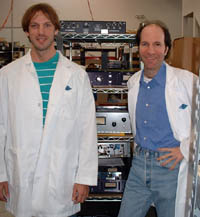
Dr. David Berners (left) is the Universal Audio Director of Algorithm Development; Dr. Jonathan Abel is the co-founder and CTO
|
Ask the Doctors: Resampling Issues
by Dave Berners
Our readers ask, "What happens when I resample my audio? Should I be worried about introducing distortion when I resample? Where in the recording process should I perform resampling?"
Resampling is essentially a filtering operation. Before resampling, a signal is represented in the discrete time by means of a series of (usually) evenly spaced samples. Provided the original continuous-time signal contains no energy above one-half the sampling frequency, the samples provide a unique representation, and the continuous-time signal can theoretically be recovered from the samples. Resampling the signal is a filtering operation whereby sample values must be computed for points in time that are not contained in the original sample set. The resampling process can thus be viewed as a calculation performed on the existing samples to interpolate the continuous-time signal. If the sampling rate is to be reduced, the bandwidth of the signal must also be reduced to one-half the new sampling rate, or aliasing will occur. Typically, in practice, the interpolation and possible bandwidth reduction are accomplished at the same time, in one filtering step.
It is important to note that resampling is a linear process. All new samples are formed as linear combinations of the existing samples (a filtering process).
Figure 1 shows a continuous-time signal (black) that has been band-limited so that it can be represented by a series of samples (blue). If the signal is to be upsampled by a factor of two, the samples shown in red must be computed based on the values of the blue samples. Note that the red samples fall directly on the (black) band-limited, continuous-time signal, which interpolates the original blue samples. Also note that, in some areas, the peak values attained by the red samples can be higher than the peaks of the blue samples. We now turn our attention to computation of the interpolating samples. What is the form of the filter that can compute the red-valued samples? Because, in this case, the red samples fall halfway between the original samples, the interpolator must introduce a one-half-sample delay.
 |
|
Figure 1. Upsampled discrete-time signal and band-limited interpolating signal.
|
For discrete-time systems, integer-sample delays are easy to produce: The data need only be stored and used at a later time. Figure 2 shows a plot of the filter transfer functions for one- and two-sample delays in black. The transfer function for a filter having a one-half sample delay is shown in red. All three filters have the same magnitude: 1.0 for frequencies below half the sampling frequency, and zero above. All three filters have linear phase, with the integer-sample-delay phases arriving at a multiple of 2π at the sampling frequency.
“It is important to note that resampling is a linear process. All new samples are formed as linear combinations of the existing samples (a filtering process).”
The zero-phase filter, which has the magnitude transfer function shown in Fig. 2, is known as the sinc function. It is computed as the Inverse Fourier Transform of the magnitude shown in Fig. 2. This function is infinite in extent, and when used as a filter, passes all frequencies up to a particular cutoff. Above the cutoff frequency, the sinc filter has infinite rejection. Figure 3 shows a plot of the sinc function. The function crosses zero at all integers other than zero. If the zeros of the function occur once every sample, the bandwidth of the filter extends to plus and minus one-half the sampling rate. The sinc function can be "stretched" in time for downsampling, so that its bandwidth becomes equal to the new sampling frequency.
 |
|
Figure 2. Magnitude and phase of ideal integer and fractional delays.
|
Sinc functions are used often for resampling. For computational purposes, some form of windowing must be applied to the function to make it finite in length, although an infinite-length sinc filter could be applied to a finite-length signal if plenty of computation is available. (This would be equivalent to applying a convolutional reverb whose length is twice the length of the audio signal.) The sinc function falls off inversely as the distance to its center, so in practice the sinc is usually truncated (after being windowed) at a point where the truncated portion is small enough to have a total power that is below the level of dither or quantization.
Computationally, the sinc filter could be used to produce the red samples of Fig. 1 in the following way: To compute a particular (red) sample, the sinc function would be centered at that sample's location. The computed value for that sample would be calculated as the sum of all of the blue samples, each having first been multiplied by the value of the sinc function at the same location (when the sinc function is centered at the sample we are trying to compute). For example, the contribution of a blue sample that is 1.5 samples away from the sample we are computing would be that sample's value times the value of sinc (1.5). This amounts to a convolution, or filtering, process.
 |
|
Figure 3. The sinc function
|
Factors affecting the precision (quality) of a sinc-based resampling algorithm include the length of the windowed sinc function (how many samples are used) and the type of window being used. One common window function for resampling is the "Kaiser" window. Typical lengths for decent-quality windowed sinc functions are on the order of 100 samples.
In terms of resampling ratios, it is more convenient to resample between sampling rates that are multiples of each other, because in that case the fractional delays that must be computed take on only a small number of values. For example, the case of Fig. 1 shows an upsampling ratio of exactly 2:1, which means that all of the computed samples interpolate the existing samples at a delay of exactly 0.5 samples. If the "to" and "from" sampling rates are not simply related, many different fractional delays must be computed during the resampling process, which means that more values for the sinc function must be known to carry out the resampling. However, there is no theoretical reason why resampling between two unrelated rates will be intrinsically worse or less accurate. The computation is simply more bulky. Competently designed resamplers can thus be used to convert between all common sampling rates equally well; there is not necessarily any quality to be gained by using only rates that are multiples of each other.
In terms of distortion, there is technically no distortion produced by resampling beyond what any other filtering would produce (round-off error). However, if the band-limiting performed by the resampling filter is inadequate, aliasing will occur. Usually, resampling filters are chosen so that the aliased components will be small enough to be beyond the limits of the number system being used.
In order to decide at what point in the mixing/mastering process to perform resampling, we will again return to Fig. 1. As mentioned earlier, it is possible that resampled data can achieve peak levels above the those of the original signal. This can occur whether the final sampling rate is higher or lower than the original. For this reason, it is usually advisable to run peak-limiting algorithms after resampling. Otherwise, the resampled data will most likely exceed the levels set in the limiting stage. However, the changes produced by resampling can have a disastrous effect on any dither that has been applied. Therefore, it is best to leave dithering until after resampling has been performed. Dither itself can also change peak levels, but only by a few LSBs for most types of dither. For 16-bit audio, at full-scale, one LSB is about one ten-thousandth of a dB. A signal that is limited to -0.1 dB will thus still be below digital full scale even after dithering. The recommended order of final processing would then be: resampling ‡ peak limiting ‡ dither. If desired, limiting could be performed before resampling, but in that case the signal would have to be renormalized to the desired peak level before dithering.
As an aside, a common topic related to resampling is peak detection in limiting, which is based on the "interpolated peaks" of a signal. Under this scheme, resampling is used in an attempt to discover the peak levels of the analog signal coming out of the D/A converters, rather than using the peak values of the signal samples themselves. This is thought to be more conservative, given that the analog headroom of the D/A is unknown. It is interesting to note that, using perfect signal reconstruction, it is possible to construct a signal whose samples all lie between plus and minus 1.0, but whose interpolated peak grows in an unbounded way as the length (in time) of the signal grows. This means that it is technically impossible to achieve true limiting on interpolated peaks, unless the peak limiter is allowed to have zero gain, in which case there is no output!